Measure Time Delays

A series of examples demonstrating various fitting options/features with SNTD.

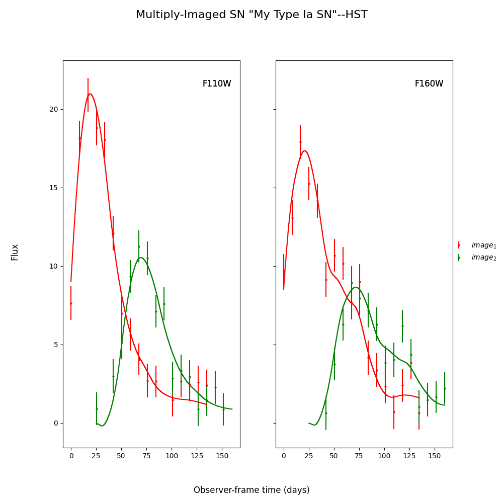
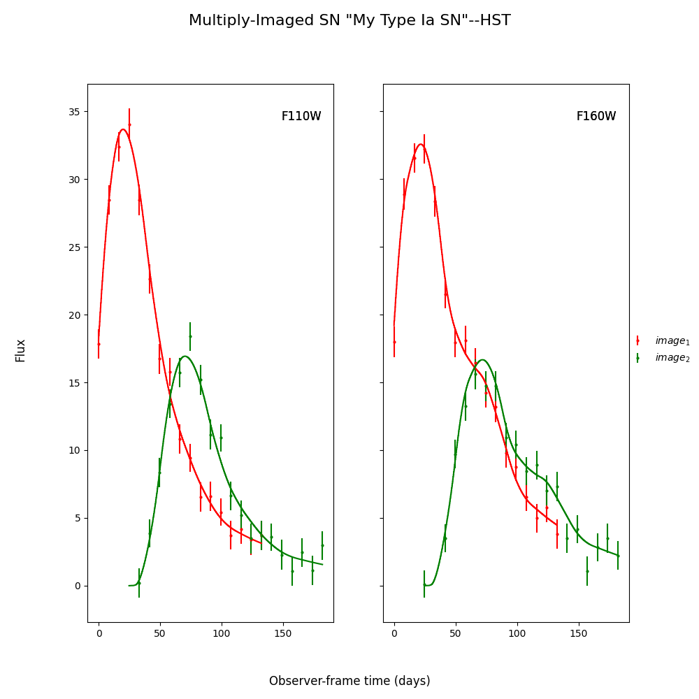
There are 3 methods built into SNTD to measure time delays (parallel, series, color). They are accessed by the same function: fit_data() . Here myMISN was generated in the Simulate Supernovae part of the documentation, using the createMultiplyImagedSN() function. The true delay for all of these fits is 50 days. You can batch process (with sbatch or multiprocessing) using any or all of these methods as well (see Batch Processing Time Delay Measurements)

Run this notebook with Google Colab.

Parallel:

import sntd

myMISN=sntd.load_example_misn()

fitCurves=sntd.fit_data(myMISN,snType='Ia', models='salt2-extended',bands=['F110W','F160W'],
                params=['x0','t0','x1','c'],constants={'z':1.4},refImage='image_1',cut_time=[-30,40],
                bounds={'t0':(-20,20),'x1':(-2,2),'c':(-1,1),'mu':(.5,2)},fitOrder=['image_1','image_2'],
                method='parallel',microlensing=None,modelcov=False,npoints=100)
print(fitCurves.parallel.time_delays)
print(fitCurves.parallel.time_delay_errors)
print(fitCurves.parallel.magnifications)
print(fitCurves.parallel.magnification_errors)
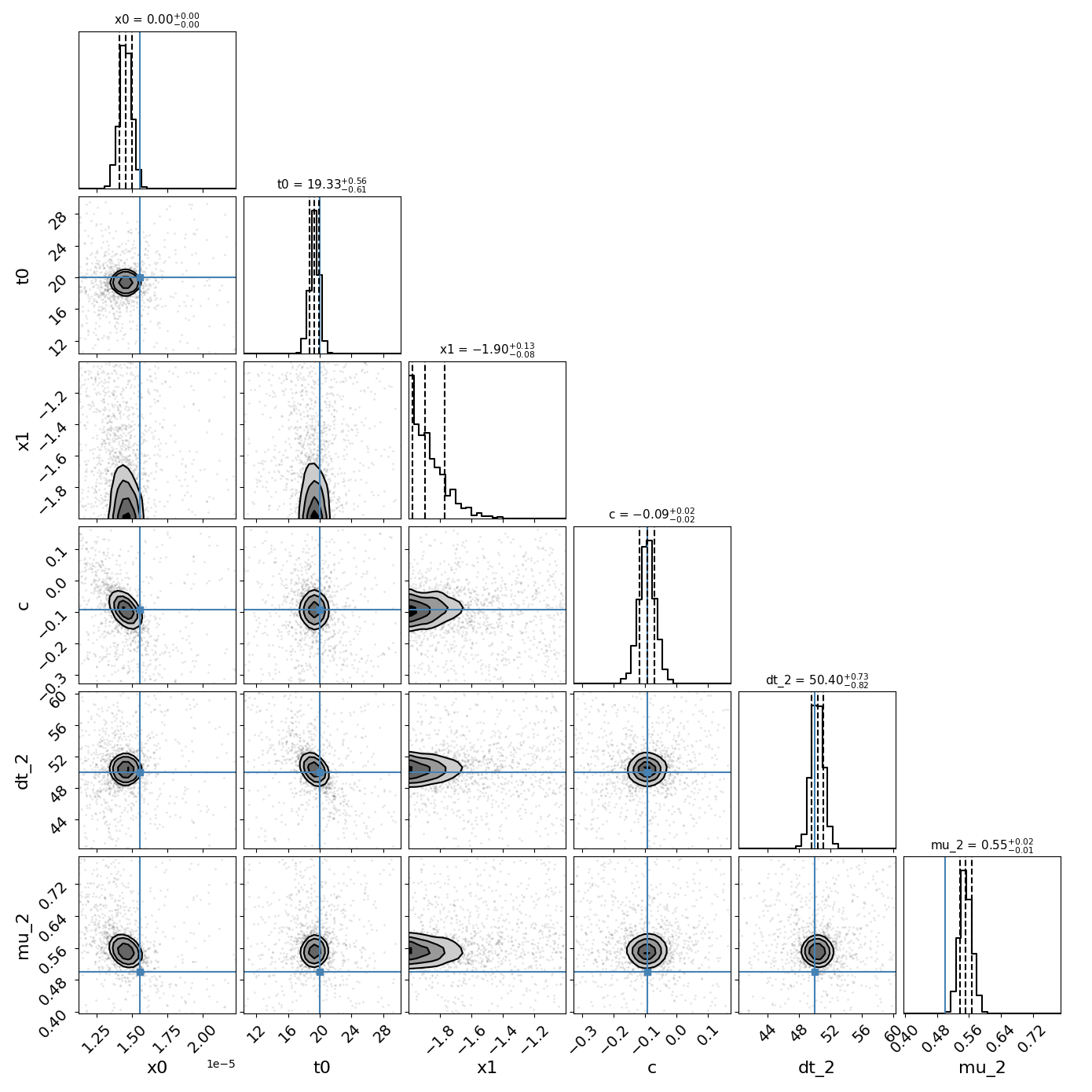
fitCurves.plot_object(showFit=True,method='parallel')
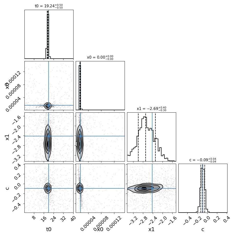
fitCurves.plot_fit(method='parallel',par_image='image_1')
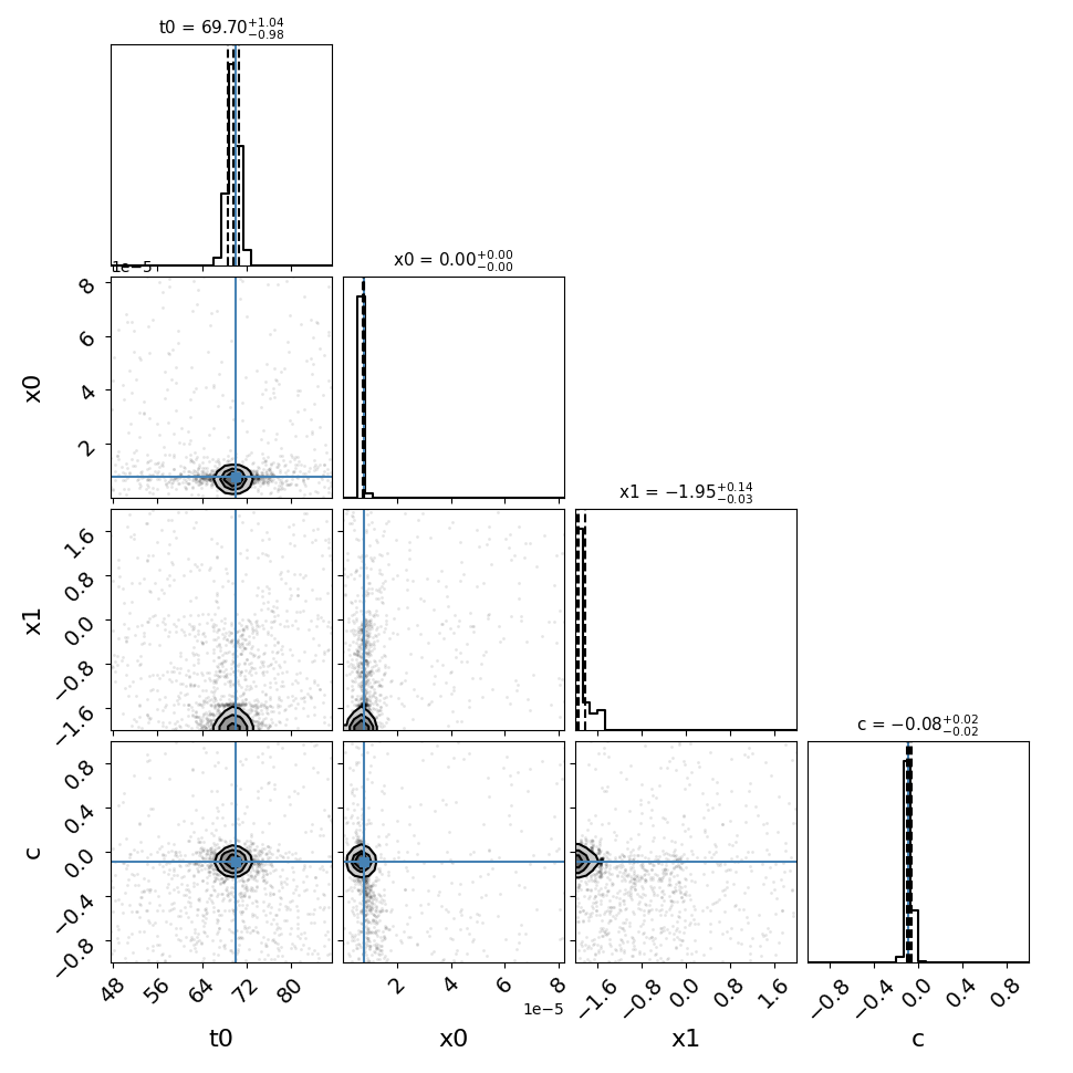
fitCurves.plot_fit(method='parallel',par_image='image_2')

• 
• 
• 

Out:

{'image_1': 0, 'image_2': 50.442299642467276}
{'image_1': array([0, 0]), 'image_2': array([-0.95826261,  0.98199374])}
{'image_1': 1, 'image_2': 0.4998899592804862}
{'image_1': array([0, 0]), 'image_2': array([-0.02284181,  0.02404375])}

<Figure size 970x970 with 16 Axes>

Note that the bounds for the ‘t0’ parameter are not absolute, the actual peak time will be estimated (unless t0_guess is defined) and the defined bounds will be added to this value. Similarly for amplitude, where bounds are multiplicative

Other methods are called in a similar fashion, with a couple of extra arguments:

Series:

fitCurves=sntd.fit_data(myMISN,snType='Ia', models='salt2-extended',bands=['F110W','F160W'],
        params=['x0','t0','x1','c'],constants={'z':1.4},refImage='image_1',cut_time=[-30,40],
        bounds={'t0':(-20,20),'td':(-20,20),'mu':(.5,2),'x1':(-2,2),'c':(-.5,.5)},
        method='series',npoints=100)


print(fitCurves.series.time_delays)
print(fitCurves.series.time_delay_errors)
print(fitCurves.series.magnifications)
print(fitCurves.series.magnification_errors)
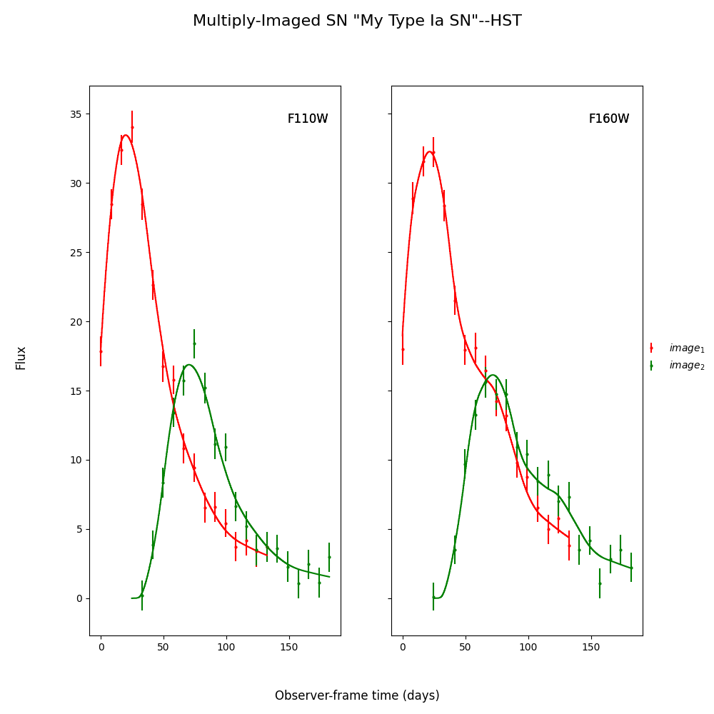
fitCurves.plot_object(showFit=True,method='series')
fitCurves.plot_fit(method='series')

• 
• 

Out:

['x0', 't0', 'x1', 'c']
['x0', 't0', 'x1', 'c']
{'image_1': 0, 'image_2': 50.39797715147582}
{'image_1': array([0, 0]), 'image_2': array([-0.82216382,  0.72853045])}
{'image_1': 1, 'image_2': 0.5515560895917695}
{'image_1': 1, 'image_2': array([-0.01397073,  0.01642504])}

<Figure size 1390x1390 with 36 Axes>

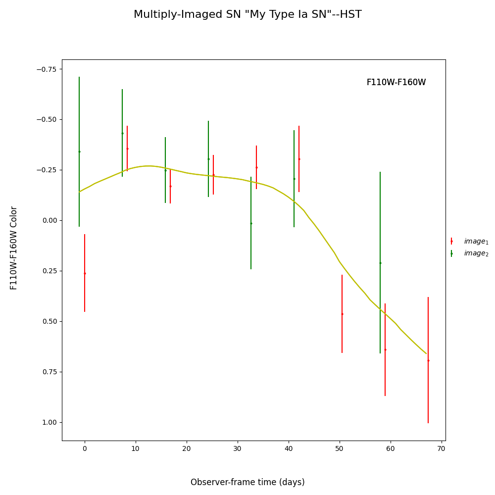
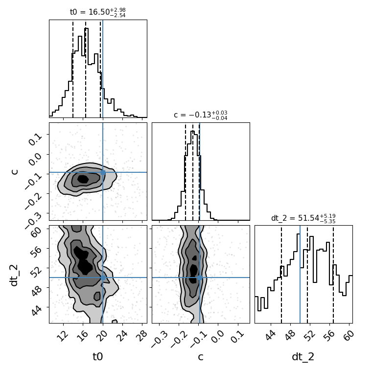
Color: By default, this will attempt to fit every combination of colors possible from the bands present in the data. You can define specific colors using the “fit_colors” argument.

fitCurves=sntd.fit_data(myMISN,snType='Ia', models='salt2-extended',bands=['F110W','F160W'],
                    params=['t0','c'],constants={'z':1.4,'x1':fitCurves.images['image_1'].fits.model.get('x1')},refImage='image_1',
                    color_param_ignore=['x1'],bounds={'t0':(-20,20),'td':(-20,20),'mu':(.5,2),'c':(-.5,.5)},cut_time=[-30,40],
                    method='color',microlensing=None,modelcov=False,npoints=200,maxiter=None,minsnr=3)

print(fitCurves.color.time_delays)
print(fitCurves.color.time_delay_errors)
fitCurves.plot_object(showFit=True,method='color')
fitCurves.plot_fit(method='color')

• 
• 

Out:

{'image_1': 0, 'image_2': 51.530224748944036}
{'image_1': array([0, 0]), 'image_2': array([-5.35065195,  5.19171365])}

<Figure size 760x760 with 9 Axes>

You can include your fit from the parallel method as a prior on light curve and time delay parameters in the series/color methods with the “fit_prior” command:

fitCurves_parallel=sntd.fit_data(myMISN,snType='Ia', models='salt2-extended',bands=['F110W','F160W'],
                    params=['x0','t0','x1','c'],constants={'z':1.4},refImage='image_1',
                    bounds={'t0':(-20,20),'x1':(-3,3),'c':(-.5,.5),'mu':(.5,2)},fitOrder=['image_1','image_2'],cut_time=[-30,40],
                        method='parallel',microlensing=None,modelcov=False,npoints=100,maxiter=None)
fitCurves_color=sntd.fit_data(myMISN,snType='Ia', models='salt2-extended',bands=['F110W','F160W'],cut_time=[-50,30],
                    params=['t0','c'],constants={'z':1.4,'x1':fitCurves.images['image_1'].fits.model.get('x1')},refImage='image_1',
                    bounds={'t0':(-20,20),'td':(-20,20),'mu':(.5,2),'c':(-.5,.5)},fit_prior=fitCurves_parallel,
                    method='color',microlensing=None,modelcov=False,npoints=200,maxiter=None,minsnr=3)

print(fitCurves_parallel.parallel.time_delays)
print(fitCurves_parallel.parallel.time_delay_errors)
print(fitCurves_color.color.time_delays)
print(fitCurves_color.color.time_delay_errors)

Out:

{'image_1': 0, 'image_2': 50.096483213906325}
{'image_1': array([0, 0]), 'image_2': array([-0.99028586,  1.26368148])}
{'image_1': 0, 'image_2': 50.31747986433648}
{'image_1': array([0, 0]), 'image_2': array([-2.01481246,  2.28440021])}

Fitting Using Extra Propagation Effects

You might also want to include other propagation effects in your fitting model, and fit relevant parameters. This can be done by simply adding effects to an SNCosmo model, in the same way as if you were fitting a single SN with SNCosmo. First we can add some extreme dust in the source and lens frames (your final simulations may look slightly different as c is chosen randomly):

myMISN2 = sntd.createMultiplyImagedSN(sourcename='salt2-extended', snType='Ia', redshift=1.4,z_lens=.53, bands=['F110W','F160W'],
              zp=[26.9,26.2], cadence=8., epochs=30.,time_delays=[20., 70.], magnifications=[20,10],
              objectName='My Type Ia SN',telescopename='HST',av_lens=1.5,
              av_host=1)
print('lensebv:',myMISN2.images['image_1'].simMeta['lensebv'],
     'hostebv:',myMISN2.images['image_1'].simMeta['hostebv'],
     'c:',myMISN2.images['image_1'].simMeta['c'])

Out:

lensebv: 0.48387096774193544 hostebv: 0.3225806451612903 c: 0.1377735187090485

Okay, now we can fit the MISN first without taking these effects into account:

fitCurves_dust=sntd.fit_data(myMISN2,snType='Ia', models='salt2-extended',bands=['F110W','F160W'],
                                                     params=['x0','x1','t0','c'],npoints=200,
                                                     constants={'z':1.4},minsnr=1,cut_time=[-30,40],
                                                     bounds={'t0':(-15,15),'x1':(-3,3),'c':(-1,1)})
print(fitCurves_dust.parallel.time_delays)
print(fitCurves_dust.parallel.time_delay_errors)
print('c:',fitCurves_dust.images['image_1'].fits.model.get('c'))
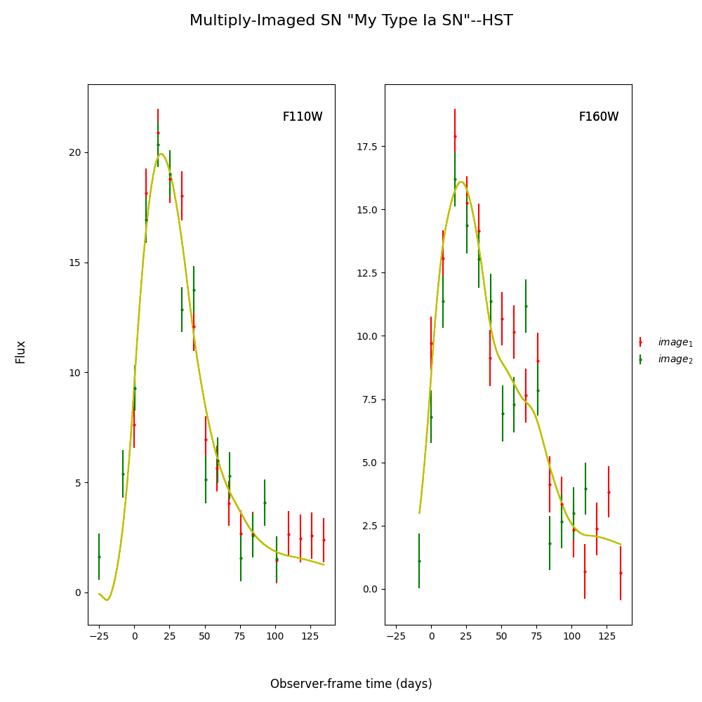
fitCurves_dust.plot_object(showFit=True)

Out:

{'image_1': 0, 'image_2': 50.412287698579206}
{'image_1': array([0, 0]), 'image_2': array([-0.74964906,  0.72983875])}
c: 0.8117704098202272

<Figure size 1000x1000 with 2 Axes>

We can see that the fitter has done reasonably well, and the time delay is still accurate (True delay is 50 days). However, one issue is that the measured value for c is vastly different than the actual value as it attempts to compensate for extinction without a propagation effect. Now let’s add in the propagation effects:

import sncosmo
dust = sncosmo.CCM89Dust()
salt2_model=sncosmo.Model('salt2-extended',effects=[dust,dust],effect_names=['lens','host'],effect_frames=['free','rest'])
fitCurves_dust=sntd.fit_data(myMISN2,snType='Ia', models=salt2_model,bands=['F110W','F160W'],npoints=200,
                    params=['x0','x1','t0','c','lensebv','hostebv'],minsnr=1,cut_time=[-30,40],
                    constants={'z':1.4,'lensr_v':3.1,'lensz':0.53,'hostr_v':3.1},
                    bounds={'t0':(-15,15),'x1':(-3,3),'c':(-.1,.1),'lensebv':(.2,1.),'hostebv':(.2,1.)})

print(fitCurves_dust.parallel.time_delays)
print(fitCurves_dust.parallel.time_delay_errors)
print('c:',fitCurves_dust.images['image_1'].fits.model.get('c'),
      'lensebv:',fitCurves_dust.images['image_1'].fits.model.get('lensebv'),
      'hostebv:',fitCurves_dust.images['image_1'].fits.model.get('hostebv'))
fitCurves_dust.plot_object(showFit=True)

Out:

{'image_1': 0, 'image_2': 50.33052950846436}
{'image_1': array([0, 0]), 'image_2': array([-0.65493107,  0.68273663])}
c: -0.30174440537013747 lensebv: -0.6076719364812484 hostebv: 1.5424337700970974

<Figure size 1000x1000 with 2 Axes>

Now the measured value for c is much closer to reality, and the measured times of peak are somewhat more accurate.