Using Your Own Data
In order to fit your own data, you must turn your light curve into an astropy table. There is an example multiply-imaged
SN example provided for reference. In this example, we have a doubly-imaged SN with image files (in the sntd/data/examples folder, what you see when running this code may be slightly different)
example_image_1.dat and example_image_2.dat. The only optional column in these files is image, which sets the name of the key
used to reference this SN image. If you do not provide flux/fluxerr but instead magnitude/magerr SNTD will attemp to translate to
flux/fluxerr, but it’s best to simply provide flux from the beginning to avoid conversion errors. First we can read in these tables:
ex_1,ex_2=sntd.load_example_data()
print(ex_1)
Out:
time         band        flux             fluxerr        zp zpsys  image
 ------------------ ----- ------------------ ------------------ --- ----- -------
                0.0 F110W   7.62584933633316 1.0755597651249478  25    AB image_1
  8.421052631578947 F110W  18.14416283987298 1.1095627479983372  25    AB image_1
 16.842105263157894 F110W  20.89546596937984 1.0789885092102118  25    AB image_1
 25.263157894736842 F110W  18.79112295341033 1.0989312899693982  25    AB image_1
  33.68421052631579 F110W  18.02156628265722   1.12828303196303  25    AB image_1
  42.10526315789473 F110W 12.085231206169226 1.1179040967533518  25    AB image_1
 50.526315789473685 F110W  6.962961065741445 1.0339735940234938  25    AB image_1
  58.94736842105263 F110W   5.62540442388384 1.0359032050500712  25    AB image_1
  67.36842105263158 F110W 4.0345924798153305   1.01660451026687  25    AB image_1
  75.78947368421052 F110W 2.6846046764855243 1.0526764468991552  25    AB image_1
                ...   ...                ...                ... ...   ...     ...
 50.526315789473685 F160W 10.672033110263037   1.05358904440353  25    AB image_1
  58.94736842105263 F160W 10.152052390226839 1.0434013477890232  25    AB image_1
  67.36842105263158 F160W 7.6435469190906415 1.0575259139938555  25    AB image_1
  75.78947368421052 F160W  9.001903536381562 1.1095984293220644  25    AB image_1
  84.21052631578947 F160W  4.136105731166709 1.1086683584388777  25    AB image_1
  92.63157894736841 F160W  3.361829966775289  1.074708117236386  25    AB image_1
 101.05263157894737 F160W 2.3313546542843953 1.0952338255910397  25    AB image_1
 109.47368421052632 F160W 0.6946360860451652  1.088838824485642  25    AB image_1
 117.89473684210526 F160W 2.3779217294236012  1.042417668422105  25    AB image_1
  126.3157894736842 F160W  3.834499918918735 1.0138401599728672  25    AB image_1
 134.73684210526315 F160W  0.623370473979624 1.0693683341393225  25    AB image_1
 Length = 33 rows
Now, to turn these two data tables into an MISN object that will be fit, we use the table_factory() function:
new_MISN=sntd.table_factory([ex_1,ex_2],telescopename='HST',object_name='example_SN')
print(new_MISN)
Out:
Telescope: HST
Object: example_SN
Number of bands: 2

------------------
Image: image_1:
Bands: {'F160W', 'F110W'}
Date Range: 0.00000->134.73684
Number of points: 33
------------------
Image: image_2:
Bands: {'F160W', 'F110W'}
Date Range: 25.26316->160.00000
Number of points: 30
------------------
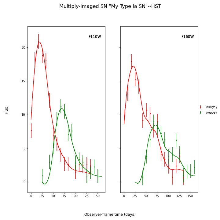
And finally let’s fit this SN, which is a Type Ia, with the SALT2 model (your exact time delay may be slightly different after fitting the example data). For reference, the true delay here is 50 days.
fitCurves=sntd.fit_data(new_MISN,snType='Ia', models='salt2-extended',bands=['F110W','F160W'],
                params=['x0','x1','t0','c'],constants={'z':1.4},
                bounds={'t0':(-25,25),'x1':(-2,2),'c':(-1,1)})
print(fitCurves.parallel.time_delays)
fitCurves.plot_object(showFit=True)
plt.show()
Out:
{'image_1': 0, 'image_2': 50.28975081972289}
Uknown Supernova Type
You may not know that your SN is a Type Ia (as other examples here and in Measure Time Delays). In that case you have two more options. You could use the parameterized Bazin model:
fitCurves=sntd.fit_data(new_MISN,snType='Ia', models='Bazin',bands=['F160W'],
            params=['t0','B','amplitude','rise','fall'],refImage='image_1',cut_time=None,
            bounds={'t0':(-20,20),'amplitude':(.1,100),'rise':(1,200),'fall':(1,200),'B':(0,1),
                   'td':(-20,20),'mu':(.5,2)},
            fitOrder=['image_1','image_2'],fit_prior=None,minsnr=3,trial_fit=True,
            method='parallel',microlensing=None,modelcov=False,npoints=100,
                        maxiter=None)
fitCurves.plot_object(showFit=True)
print(fitCurves.parallel.time_delays)
Out:
{'image_1': 0, 'image_2': 49.40967718450336}
Another option is to fit multiple models from different SN types. SNTD will choose the “best” model using the Bayesian Evidence.
fitCurves=sntd.fit_data(new_MISN,snType='Ia', models=['salt2-extended','hsiao','snana-2004gq',
    'snana-2004fe','snana-2004gv','snana-2007nc'],
    bands=['F110W','F140W'],cut_time=[-500,30],
    params=['x0','t0','x1','c','amplitude'],constants={'z':1.33},refImage='image_1',
    bounds={'t0':(-20,20),'x1':(-3,3),'c':(-1,1),'td':(-20,20),'mu':(.5,2)},
    fitOrder=['image_2','image_1'],trial_fit=True,minsnr=3,
    method='parallel',microlensing=None,modelcov=False,npoints=50,clip_data=True,
    maxiter=None)
Batch Processing Time Delay Measurements
Parallel processing and batch processing is built into SNTD in order to fit a large number of (likely simulated) MISN. To access this feature,
simply provide a list of MISN instead of a single MISN object, specifying whether you want to use multiprocessing (split the list across multiple cores)
or batch processing (splitting the list into multiple jobs with sbatch). If you specify batch mode, you need to provide
the partition and number of jobs you want to implement or the number of lensed SN you want to fit per node.
myMISN1 = sntd.createMultiplyImagedSN(sourcename='salt2-extended', snType='Ia', redshift=1.33,z_lens=.53, bands=['F110W','F125W'],
                 zp=[26.8,26.2], cadence=5., epochs=35.,time_delays=[10., 70.], magnifications=[7,3.5],
     objectName='My Type Ia SN',telescopename='HST')
myMISN2 = sntd.createMultiplyImagedSN(sourcename='salt2-extended', snType='Ia', redshift=1.33,z_lens=.53, bands=['F110W','F125W'],
                 zp=[26.8,26.2], cadence=5., epochs=35.,time_delays=[10., 50.], magnifications=[7,3.5],
     objectName='My Type Ia SN',telescopename='HST')
curve_list=[myMISN1,myMISN2]
fitCurves=sntd.fit_data(curve_list,snType='Ia', models='salt2-extended',bands=['F110W','F125W'],
                  params=['x0','t0','x1','c'],constants={'z':1.3},refImage='image_1',
                  bounds={'t0':(-20,20),'x1':(-3,3),'c':(-1,1)},fitOrder=['image_2','image_1'],
                  method='parallel',npoints=1000,par_or_batch='batch', batch_partition='myPartition',nbatch_jobs=2)

for curve in fitCurves:
  print(curve.parallel.time_delays)

fitCurves=sntd.fit_data(curve_list,snType='Ia', models='salt2-extended',bands=['F110W','F125W'],
                  params=['x0','t0','x1','c'],constants={'z':1.3},refImage='image_1',
                  bounds={'t0':(-20,20),'x1':(-3,3),'c':(-1,1)},fitOrder=['image_2','image_1'],
                  method='parallel',npoints=1000,par_or_batch='parallel')
for curve in fitCurves:
  print(curve.parallel.time_delays)
Out:
Submitted batch job 5784720
{'image_1': 0, 'image_2': 60.3528844834}
{'image_1': 0, 'image_2': 40.34982372733}
Fitting MISN number 1...
Fitting MISN number 2...
{'image_1': 0, 'image_2': 60.32583528844834}
{'image_1': 0, 'image_2': 40.22834982372733}
You can also use batch processing and multiprocssing (using N cores per node across M cores using Slurm):
fitCurves=sntd.fit_data(curve_list,snType='Ia', models='salt2-extended',bands=['F110W','F125W'],
            params=['x0','t0','x1','c'],constants={'z':1.3},refImage='image_1',
            bounds={'t0':(-20,20),'x1':(-3,3),'c':(-1,1)},fitOrder=['image_2','image_1'],n_cores_per_node=2,
            method='parallel',npoints=1000,par_or_batch='batch', batch_partition='myPartition',nbatch_jobs=1)
If you would like to run multiple methods in a row in batch mode, the recommended way is by providing a list of the methods to the fit_data() function. You
can have it use the parallel fit as a prior on the subsequent fits by setting fit_prior to True instead of giving it a MISN object.
fitCurves_batch=sntd.fit_data(curve_list,snType='Ia', models='salt2-extended',bands=['F110W','F125W'],
                  params=['x0','t0','x1','c'],constants={'z':1.3},refImage='image_1',fit_prior=True,
                  bounds={'t0':(-20,20),'x1':(-3,3),'c':(-1,1)},fitOrder=['image_2','image_1'],
                  method=['parallel','series','color'],npoints=1000,par_or_batch='batch', batch_partition='myPartition',nbatch_jobs=2)
Fitting Model Params Only
You can also easily fix the time delays (for the series or color method) and/or magnifications (series method only) while fitting a light curve model:
myMISN = sntd.load_example_misn()
fitCurves=sntd.fit_data(myMISN,snType='Ia',models='salt2-extended',bands=['F110W','F160W'],
                      params=['x0','x1','t0','c'],constants={'z':1.4,'td':{'image_1':0,'image_2':50}},
                      refImage='image_1',trial_fit=False,
                      bounds={'t0':(-20,20),'mu':(.5,2),'x1':(-2,2),'c':(-.5,.5)},
                      method='series',npoints=100)
print(fitCurves.series.time_delays)
print(fitCurves.series.magnifications)
fitCurves.plot_fit(method='series')
plt.show()
Out:
{'image_1': 0, 'image_2': 50}
{'image_1': 1, 'image_2': 0.5496620676889558}
myMISN = sntd.load_example_misn()
fitCurves=sntd.fit_data(myMISN,snType='Ia',models='salt2-extended',bands=['F110W','F160W'],
                      params=['x0','x1','t0','c'],constants={'z':1.4,'mu':{'image_1':1,'image_2':0.5}},
                      refImage='image_1',trial_fit=False,
                      bounds={'t0':(-20,20),'mu':(.5,2),'x1':(-2,2),'c':(-.5,.5)},
                      method='series',npoints=100)
print(fitCurves.series.time_delays)
print(fitCurves.series.magnifications)
fitCurves.plot_fit(method='series')
plt.show()
Out:
{'image_1': 0, 'image_2': 50.29975290189155}
{'image_1': 1, 'image_2': 0.5}
myMISN = sntd.load_example_misn()
fitCurves=sntd.fit_data(myMISN,snType='Ia',models='salt2-extended',bands=['F110W','F160W'],
                      params=['x0','x1','t0','c'],constants={'z':1.4,'td':{'image_1':0,'image_2':50},'mu':{'image_1':1,'image_2':0.5}},
                      refImage='image_1',trial_fit=False,
                      bounds={'t0':(-20,20),'mu':(.5,2),'x1':(-2,2),'c':(-.5,.5)},
                      method='series',npoints=100)
print(fitCurves.series.time_delays)
print(fitCurves.series.magnifications)
fitCurves.plot_fit(method='series')
plt.show()
Out:
{'image_1': 0, 'image_2': 50}
{'image_1': 1, 'image_2': 0.5}
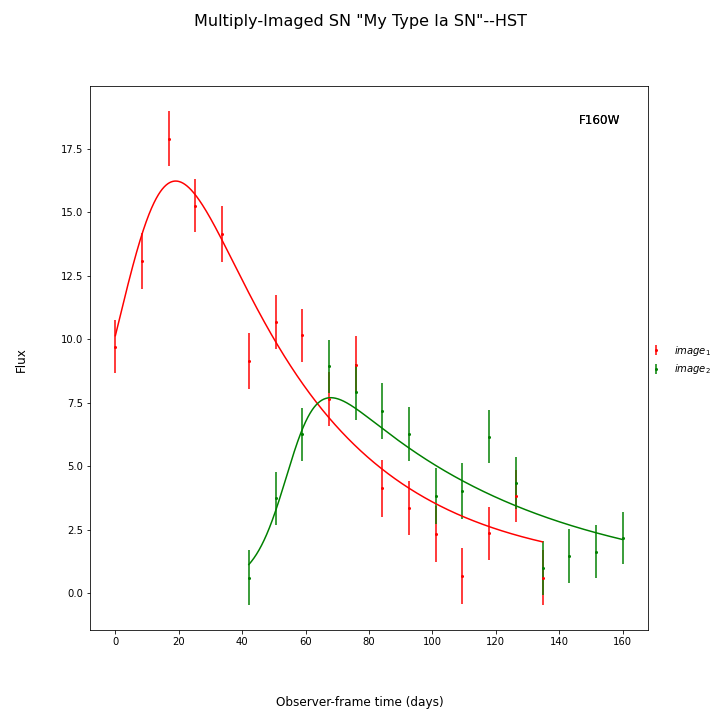
Unresolved Lensed SN Models
SNTD now includes an option for fitting unresolved multiply-imaged light curves. Here is an example of an unresolved light curve of a doubly-imaged SN Ia:
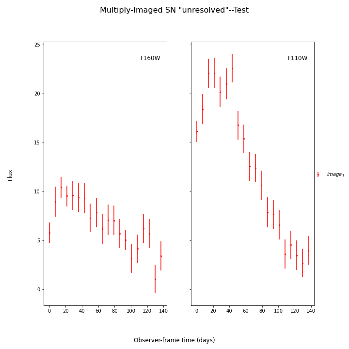
This object has only a single image, whose table is the combined light curve shown above. Simply create SNCosmo models for each blended image, and combine them in the following way:
image_1 = sncosmo.Model('salt2-extended')
image_2 = sncosmo.Model('salt2-extended')
unresolved=sntd.unresolvedMISN([image_1,image_2])
You can set the time delays and magnifications with two simple functions:
unresolved.set_delays([20,55])
unresolved.set_magnifications([4,1])
print(unresolved.model_list[0].parameters)
print(unresolved.model_list[1].parameters)
Out:
[ 0. 20. 4. 0. 0. ]
[ 0. 55. 1. 0. 0. ]
You may now set parameters as you would for a normal model. SN parameters (i.e. z, x1, c, etc.) will set across all models, “lens” parameters (i.e. t0, x0/amplitude, etc.) will shift each model by that amount. For example (note the time delays above):
unresolved.set(z=1.4)
unresolved.set(t0=10)
print(unresolved.param_names)
print(unresolved.parameters)
print(unresolved.model_list[0].parameters)
print(unresolved.model_list[1].parameters)
Out:
['z', 't0', 'x0', 'x1', 'c', 'dt_1', 'mu_1', 'dt_2', 'mu_2']
[ 1.4 10.   1.   0.   0. 20. 4. 55. 1. ]
[ 1.4 30.   4.   0.   0. ]
[ 1.4 65.   1.   0.   0. ]
Now this unresolved model can be simply used in the SNTD fitting methods as normal:
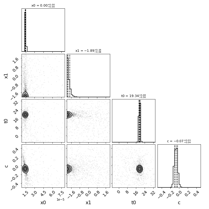
fitCurves=sntd.fit_data(combined_MISN,snType='Ia',models=unresolved,bands=['F110W','F160W'],
                        params=['x0','x1','t0','c'],constants={'z':1.4},
                        bounds={'t0':(-20,20),'x1':(-2,2),'c':(-.5,.5)},
                        method='parallel',npoints=100)

print(list(zip(fitCurves.images['image_1'].fits.model.param_names,
  fitCurves.images['image_1'].fits.model.parameters)))
fitCurves.plot_object(showFit=True,plot_unresolved=True)
plt.show()
Out:
[('z', 1.4), ('t0', -0.7620832162021888), ('x0', 7.298888590029448e-07), ('x1', 1.4960457248192203), ('c', -0.08384340717738858), ('dt_1', 20.0), ('mu_1', 4.0), ('dt_2', 55.0), ('mu_2', 1.0)]
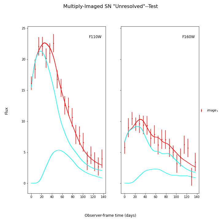
Here the true parameters were t0=0 (the input time delays were correct, and t0 is fitting for a global offset in the model), x1=-1.33, c=-.02, and x0 is somewhat arbitrary here as the magnifications were also correct based on the sim.
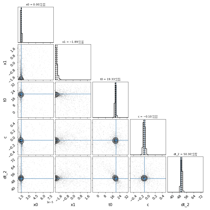
Additionally, we can attempt to fit for relative time delays/magnifications of the unresolved images.
fitCurves=sntd.fit_data(combined_MISN,snType='Ia',models=unresolved,bands=['F110W','F160W'],
                        params=['x0','x1','t0','c','dt_2'],
                        constants={'z':1.4,'mu_1':2,'mu_2':.5},
                        bounds={'t0':(-20,20),'dt_2':(20,40),'x1':(-2,2),'c':(-.5,.5)},
                        method='parallel',npoints=100)

print(list(zip(fitCurves.images['image_1'].fits.model.param_names,
  fitCurves.images['image_1'].fits.model.parameters)))
fitCurves.plot_object(showFit=True,plot_unresolved=True)
plt.show()
Out:
[('z', 1.4), ('t0', 19.203237085466867), ('x0', 7.349261421179482e-07), ('x1', 1.682206180032783), ('c', -0.0909991294403899), ('dt_1', 0.0), ('mu_1', 4.0), ('dt_2', 38.205546125150704), ('mu_2', 1.0)]

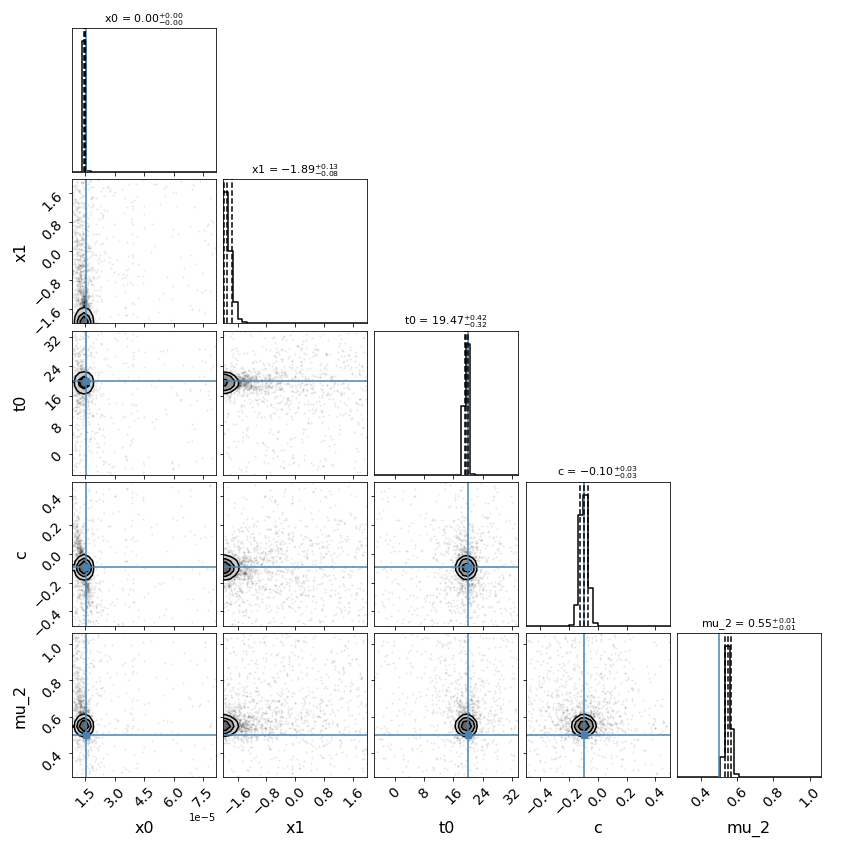
fitCurves=sntd.fit_data(combined_MISN,snType='Ia',models=unresolved,bands=['F110W','F160W'],
                        params=['x0','x1','t0','c','mu_1',dt_2','mu_2'],
                        constants={'z':1.4},
                        bounds={'t0':(-20,20),'mu_1':(3.5,4.5),'mu_2':(.5,1.5),
                                        'dt_2':(20,80),'x1':(-3,3),'c':(-.5,.5)},
                        method='parallel',npoints=100)

print(list(zip(fitCurves.images['image_1'].fits.model.param_names,
  fitCurves.images['image_1'].fits.model.parameters)))
fitCurves.plot_object(showFit=True,plot_unresolved=True)
fitCurves.plot_fit()
plt.show()
Out:
[('z', 1.4), ('t0', 19.49243682866722), ('x0', 7.43527262511094e-07), ('x1', 1.7221753624460694), ('c', -0.08879485874943827), ('dt_1', 0.0), ('mu_1', 3.980681598438305), ('dt_2', 38.91567004151568), ('mu_2', 0.9718061929858269)]

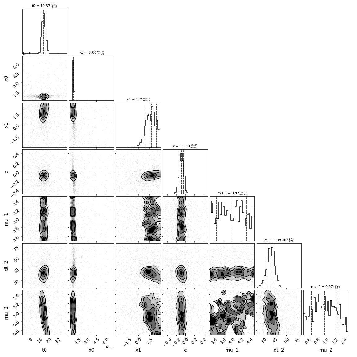
For these last two examples, there is a lot of parameter degeneracy but we still do reasonably well. The true values are t0=20,dt_2=35,mu_1=4,mu_2=1, c=-0.02., x1=1.33.
Note that you can add individual propagation effects to each images model at the outset (such as lens plane dust or microlensing models), or you could add a single propagation effect to the unresolved model that will impact the combined model (such as host galaxy dust):
dust = sncosmo.F99Dust()
image_1 = sncosmo.Model('salt2-extended',effects=[dust],
                                   effect_names=['lens_1'],
                                   effect_frames=['free'])
image_2 = sncosmo.Model('salt2-extended')
unresolved=sntd.unresolvedMISN([image_1,image_2])
print(list(zip(unresolved.param_names,unresolved.parameters)))
Out:
[('z', 0.0), ('t0', 0.0), ('x0', 1.0), ('x1', 0.0), ('c', 0.0), ('lens_1z', 0.0), ('lens_1ebv', 0.0), ('lens_1r_v', 3.1), ('dt_1', 0.0), ('mu_1', 1.0), ('dt_2', 0.0), ('mu_2', 1.0)]
unresolved.set(lens_1ebv=.5)
print(unresolved.get('lens_1ebv'))
unresolved.add_effect(dust,'host','rest')
print(list(zip(unresolved.param_names,unresolved.parameters)))
unresolved.set(hostebv=.3)
print(unresolved.get('hostebv'))
print(unresolved.model_list[0].effect_names)
Out:
0.5
[('z', 0.0), ('t0', 0.0), ('x0', 1.0), ('x1', 0.0), ('c', 0.0), ('lens_1z', 0.0), ('lens_1ebv', 0.5), ('lens_1r_v', 3.1), ('dt_1', 0.0), ('mu_1', 1.0), ('dt_2', 0.0), ('mu_2', 1.0), ('hostebv', 0.0), ('hostr_v', 3.1)]
0.3
['lens_1', 'host']
Note that the number of parameters is getting extremely long (and this is only 2 images!), so it’s recommended to fix as many of these parameters by other means as possible (i.e., the dust parameters will be difficult to constrain simultaneously with the light curve and time delay parameters).