Microlensing Analysis

Simulate and fit for microlensing.

This notebook gives examples on creating microlensing for simulations, including microlensing in light curves, and fitting for a microlensing uncertainty.

Run this notebook with Google Colab.

import sntd
import numpy as np
from sklearn.gaussian_process.kernels import RBF
np.random.seed(3)

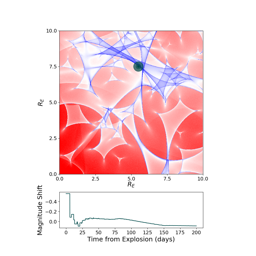
myML=sntd.realizeMicro(nray=100,kappas=1,kappac=.3,gamma=.4)
time,dmag=sntd.microcaustic_field_to_curve(field=myML,time=np.arange(0,200,.1),zl=.5,zs=1.5,plot=True,loc=[550,750])

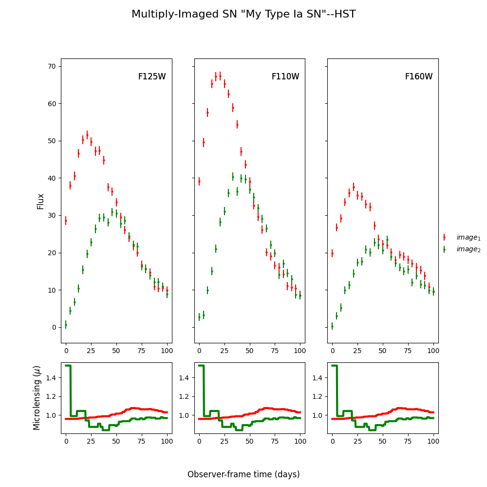
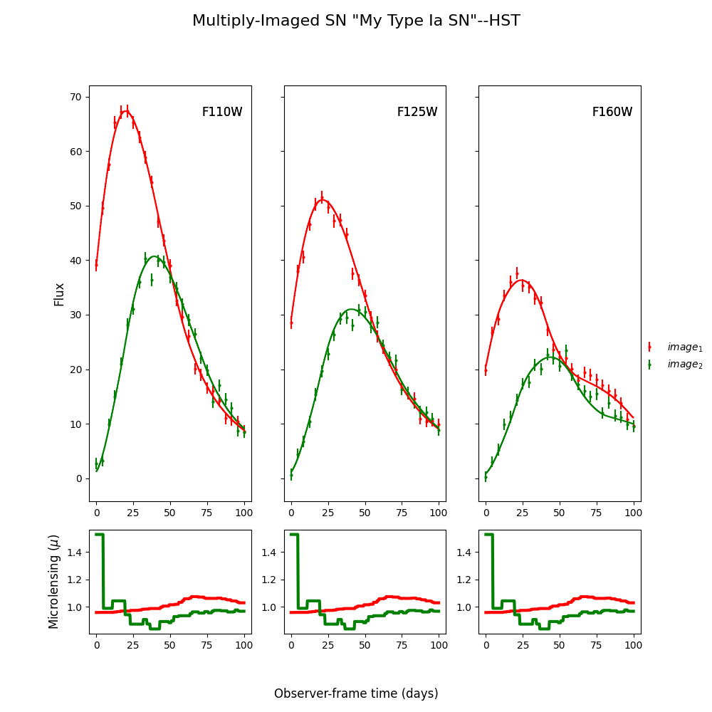
Including Microlensing in Simulations Now we can take the simulated microcaustic and use it to include microlensing in a multiply-imaged supernova simulation. See the Simulate Supernovae example for more simulation details.

myMISN = sntd.createMultiplyImagedSN(sourcename='salt2-extended', snType='Ia', redshift=1.5,z_lens=.5, bands=['F110W','F125W','F160W'],
        zp=[26.8,26.5,26.2], cadence=4., epochs=25.,time_delays=[20., 40.], magnifications=[12,8],ml_loc=[[600,800],[550,750]],
        objectName='My Type Ia SN',telescopename='HST', microlensing_type='AchromaticMicrolensing',microlensing_params=myML)
myMISN.plot_object(showMicro=True)

Out:

<Figure size 1000x1000 with 6 Axes>

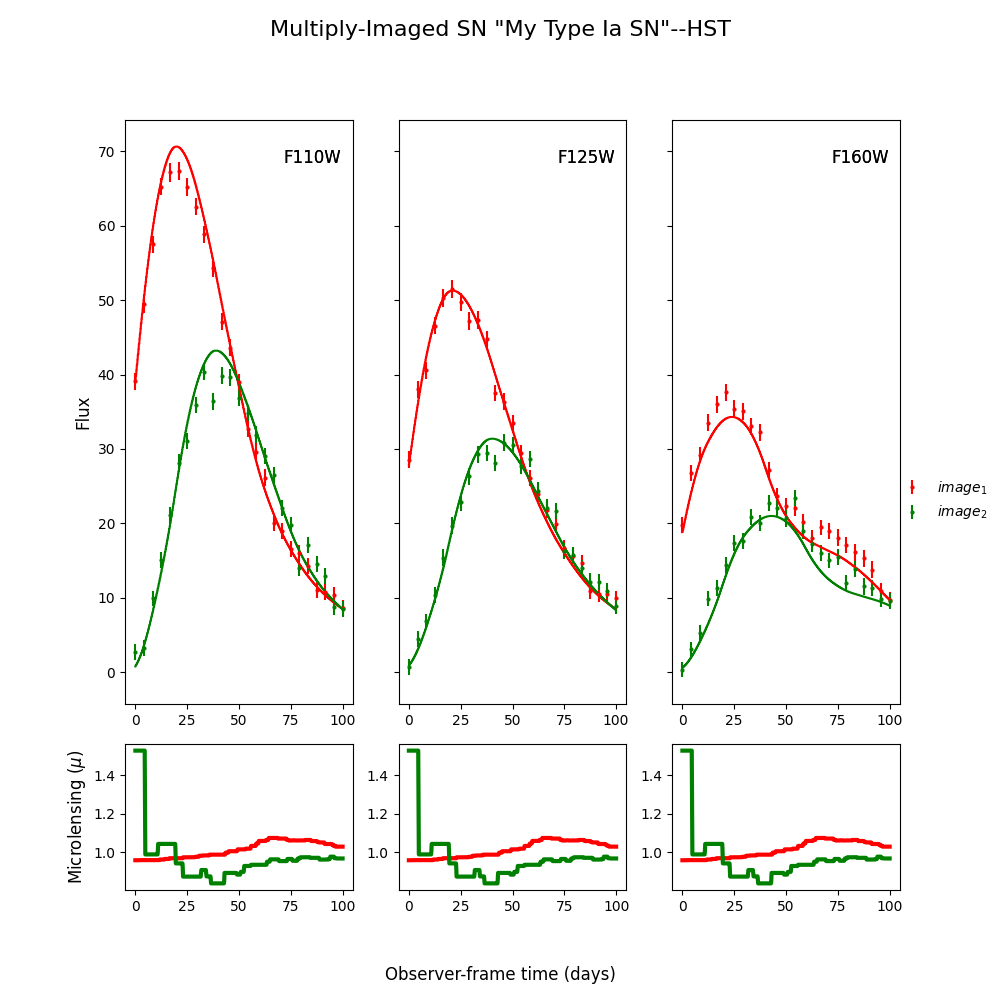
Measuring Addition Microlensing Uncertainty Now we can take the simulated light curve with microlensing and fit for an additional microlensing uncertainty term. See the Measure Time Delays example for fitting details. We start by assuming the correct shape/color parameters.

fitCurves = sntd.fit_data(myMISN, snType='Ia', models='salt2-extended', bands=['F110W','F125W', 'F160W'],
                                  params=['x0', 't0'],
                                  constants={'z': 1.5,'x1':myMISN.images['image_1'].simMeta['x1'],'c':myMISN.images['image_1'].simMeta['c']},
                                  bounds={'t0': (-40, 40),'c': (-1, 1), 'x1': (-2, 2), },
                                  method='parallel', microlensing='achromatic',
                                  nMicroSamples=40, npoints=100, minsnr=5,kernel=RBF(1.,(.0001,1000)))
print('Time Delays:',fitCurves.parallel.time_delays)
fitCurves.plot_object(showFit=True,showMicro=True)
for image in fitCurves.images.keys():
    print(image,'Microlensing Uncertainty:',fitCurves.images[image].param_quantiles['micro'],' Days')

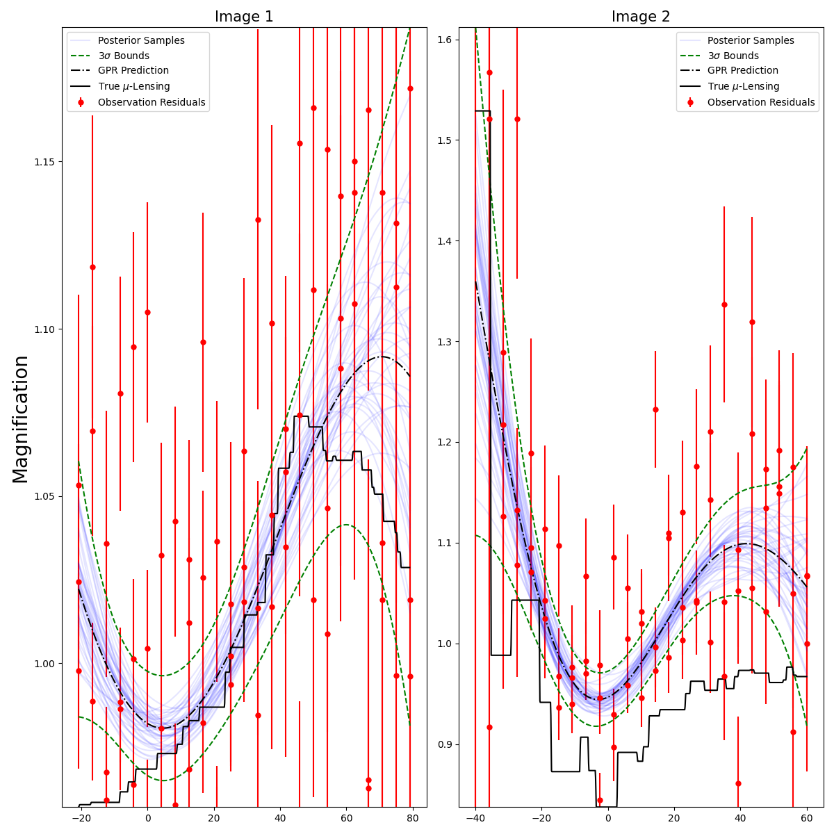
fitCurves.plot_microlensing_fit(show_all_samples=True)

• 
• 

Out:

Time Delays: {'image_1': 0, 'image_2': 19.10361601481741}
image_1 Microlensing Uncertainty: 0.010268162214037983  Days
image_2 Microlensing Uncertainty: 0.028788219176668055  Days

(<Figure size 1200x1200 with 2 Axes>, [])

We see that this extra uncertainty is quite small here, and indeed when fitting for x1/c as well, the time delay measurement is very close to the true value of 20 days.

fitCurves = sntd.fit_data(myMISN, snType='Ia', models='salt2-extended', bands=['F110W','F125W', 'F160W'],
                                  params=['x0', 't0','x1','c'],
                                  constants={'z': 1.5},
                                  bounds={'t0': (-40, 40),'c': (-1, 1), 'x1': (-2, 2)},
                                  method='parallel', microlensing=None,
                                  npoints=100, minsnr=5)
print('Time Delays:',fitCurves.parallel.time_delays)
fitCurves.plot_object(showFit=True,showMicro=True)

Out:

Time Delays: {'image_1': 0, 'image_2': 19.55887430479142}

<Figure size 1000x1000 with 6 Axes>